Analyzing circadian transcriptome data with LimoRhyde
2026-01-20
Source:vignettes/introduction.Rmd
introduction.RmdLimoRhyde is a framework for differential analysis of rhythmic transcriptome data. This vignette goes through the typical steps of an analysis: identifying rhythmic genes, identifying differentially rhythmic genes, and identifying differentially expressed genes.
The dataset is based on total RNA from livers of wild-type and Rev-erb knockout mice, with gene expression measured by microarray (GSE34018).
Load packages and set parameters
library('annotate')
library('data.table')
library('foreach')
library('ggplot2')
library('limma')
library('limorhyde')
library('org.Mm.eg.db')
Here we specify the zeitgeber period and the q-value cutoffs for rhythmic and differentially rhythmic genes.
period = 24
qvalRhyCutoff = 0.15
qvalDrCutoff = 0.1
Load the data
The expression data are in a matrix with one row per gene and one column per sample. The metadata are in a table with one row per sample.
y = readRDS(system.file('extdata', 'GSE34018_expression_data.rds', package = 'limorhyde'))
y[1:5, 1:5]
#>       GSM840516 GSM840517 GSM840518 GSM840519 GSM840520
#> 11287  7.985859  7.930935  7.674688  7.899531  7.768563
#> 11298  7.719384  7.737210  7.888502  7.865563  7.772749
#> 11302 12.594006 12.557148 11.754031 11.851858 11.656702
#> 11303  7.868566  7.823121  7.907136  7.906957  7.934719
#> 11304  7.772076  7.930239  7.774563  7.768792  7.740474

metadata = readRDS(system.file('extdata', 'GSE34018_metadata.rds', package = 'limorhyde'))
metadata
#>     sample_id                                  title              genotype
#>        <char>                                 <char>                <char>
#>  1: GSM840516              wild-type liver_ZT0_rep 1             wild-type
#>  2: GSM840517              wild-type liver_ZT0_rep 2             wild-type
#>  3: GSM840518              wild-type liver_ZT4_rep 1             wild-type
#>  4: GSM840519              wild-type liver_ZT4_rep 2             wild-type
#>  5: GSM840520              wild-type liver_ZT8_rep 1             wild-type
#>  6: GSM840521              wild-type liver_ZT8_rep 2             wild-type
#>  7: GSM840522             wild-type liver_ZT12_rep 1             wild-type
#>  8: GSM840523             wild-type liver_ZT12_rep 2             wild-type
#>  9: GSM840524             wild-type liver_ZT16_rep 1             wild-type
#> 10: GSM840525             wild-type liver_ZT16_rep 2             wild-type
#> 11: GSM840526             wild-type liver_ZT20_rep 1             wild-type
#> 12: GSM840527             wild-type liver_ZT20_rep 2             wild-type
#> 13: GSM840504  Reverb alpha/beta DKO liver_ZT0_rep 1 Reverb alpha/beta DKO
#> 14: GSM840505  Reverb alpha/beta DKO liver_ZT0_rep 2 Reverb alpha/beta DKO
#> 15: GSM840506  Reverb alpha/beta DKO liver_ZT4_rep 1 Reverb alpha/beta DKO
#> 16: GSM840507  Reverb alpha/beta DKO liver_ZT4_rep 2 Reverb alpha/beta DKO
#> 17: GSM840508  Reverb alpha/beta DKO liver_ZT8_rep 1 Reverb alpha/beta DKO
#> 18: GSM840509  Reverb alpha/beta DKO liver_ZT8_rep 2 Reverb alpha/beta DKO
#> 19: GSM840510 Reverb alpha/beta DKO liver_ZT12_rep 1 Reverb alpha/beta DKO
#> 20: GSM840511 Reverb alpha/beta DKO liver_ZT12_rep 2 Reverb alpha/beta DKO
#> 21: GSM840512 Reverb alpha/beta DKO liver_ZT16_rep 1 Reverb alpha/beta DKO
#> 22: GSM840513 Reverb alpha/beta DKO liver_ZT16_rep 2 Reverb alpha/beta DKO
#> 23: GSM840514 Reverb alpha/beta DKO liver_ZT20_rep 1 Reverb alpha/beta DKO
#> 24: GSM840515 Reverb alpha/beta DKO liver_ZT20_rep 2 Reverb alpha/beta DKO
#>     sample_id                                  title              genotype
#>        <char>                                 <char>                <char>
#>      time      cond
#>     <num>    <fctr>
#>  1:     0 wild-type
#>  2:     0 wild-type
#>  3:     4 wild-type
#>  4:     4 wild-type
#>  5:     8 wild-type
#>  6:     8 wild-type
#>  7:    12 wild-type
#>  8:    12 wild-type
#>  9:    16 wild-type
#> 10:    16 wild-type
#> 11:    20 wild-type
#> 12:    20 wild-type
#> 13:     0  knockout
#> 14:     0  knockout
#> 15:     4  knockout
#> 16:     4  knockout
#> 17:     8  knockout
#> 18:     8  knockout
#> 19:    12  knockout
#> 20:    12  knockout
#> 21:    16  knockout
#> 22:    16  knockout
#> 23:    20  knockout
#> 24:    20  knockout
#>      time      cond
#>     <num>    <fctr>
We use limorhyde to calculate time_cos and
time_sin, which are based on the first harmonic of a
Fourier decomposition of the time column, and append them
to the metadata data.table.
Identify rhythmic genes
The next three steps use limma. We calculate the q-value of rhythmicity for each gene using that gene’s p-value for each condition and adjusting for multiple testing.
rhyLimma = foreach(condNow = unique(metadata$cond), .combine = rbind) %do% {
  design = model.matrix(~ time_cos + time_sin, data = metadata[cond == condNow])
  fit = lmFit(y[, metadata$cond == condNow], design)
  fit = eBayes(fit, trend = TRUE)
  rhyNow = data.table(topTable(fit, coef = 2:3, number = Inf), keep.rownames = TRUE)
  setnames(rhyNow, 'rn', 'gene_id')
  rhyNow[, cond := condNow]}

rhyLimmaSummary = rhyLimma[, .(P.Value = min(P.Value)), by = gene_id]
rhyLimmaSummary[, adj.P.Val := p.adjust(P.Value, method = 'BH')]
setorderv(rhyLimmaSummary, 'adj.P.Val')

rhyLimmaSummary[1:5, ]
#>    gene_id      P.Value    adj.P.Val
#>     <char>        <num>        <num>
#> 1:   13170 7.783218e-15 1.334277e-10
#> 2:  353187 2.580065e-12 2.211503e-08
#> 3:   15496 4.322474e-12 2.470005e-08
#> 4:   12700 1.536660e-11 6.585740e-08
#> 5:  321018 2.628480e-11 9.012007e-08
Identify differentially rhythmic genes
Differential rhythmicity is based on statistical interactions between
cond and the time components. We pass all
genes to limma (whose Empirical Bayes does best with many genes), but
keep results only for rhythmic genes, and adjust for multiple testing
accordingly.
design = model.matrix(~ cond * (time_cos + time_sin), data = metadata)

fit = lmFit(y, design)
fit = eBayes(fit, trend = TRUE)
drLimma = data.table(topTable(fit, coef = 5:6, number = Inf), keep.rownames = TRUE)
setnames(drLimma, 'rn', 'gene_id')

drLimma = drLimma[gene_id %in% rhyLimmaSummary[adj.P.Val <= qvalRhyCutoff]$gene_id]
drLimma[, adj.P.Val := p.adjust(P.Value, method = 'BH')]
setorderv(drLimma, 'adj.P.Val')

drLimma[1:5, ]
#>    gene_id condknockout.time_cos condknockout.time_sin   AveExpr        F
#>     <char>                 <num>                 <num>     <num>    <num>
#> 1:   12686            -1.5326997           -0.04338787 10.157657 63.69962
#> 2:  353187             0.6825313           -0.35398532  9.422013 63.33021
#> 3:  270166            -1.0453062            0.26766077 12.112605 57.37334
#> 4:  207818            -0.6412353           -0.15187573 10.482197 57.04975
#> 5:   15486            -0.7315828            0.12824401 12.503645 44.83717
#>         P.Value    adj.P.Val
#>           <num>        <num>
#> 1: 9.697947e-11 2.416131e-07
#> 2: 1.032534e-10 2.416131e-07
#> 3: 2.965555e-10 3.683675e-07
#> 4: 3.148440e-10 3.683675e-07
#> 5: 3.788290e-09 3.545840e-06
Identify differentially expressed genes
Differential expression is based on the coefficient for
cond in a linear model with no interaction terms. We pass
all genes to limma, but keep results only for non-differentially
rhythmic genes, and adjust for multiple testing accordingly.
design = model.matrix(~ cond + time_cos + time_sin, data = metadata)

fit = lmFit(y, design)
fit = eBayes(fit, trend = TRUE)
deLimma = data.table(topTable(fit, coef = 2, number = Inf), keep.rownames = TRUE)
setnames(deLimma, 'rn', 'gene_id')

deLimma = deLimma[!(gene_id %in% drLimma[adj.P.Val <= qvalDrCutoff]$gene_id)]
deLimma[, adj.P.Val := p.adjust(P.Value, method = 'BH')]
setorderv(deLimma, 'adj.P.Val')

deLimma[1:5, ]
#>    gene_id     logFC   AveExpr         t      P.Value    adj.P.Val        B
#>     <char>     <num>     <num>     <num>        <num>        <num>    <num>
#> 1:   11302 -2.271205 11.260315 -23.07298 1.343920e-19 2.076357e-15 33.11228
#> 2:   68680 -1.653067  9.096748 -18.20762 6.316866e-17 4.879779e-13 27.87922
#> 3:   67442 -1.208461 14.375311 -16.67075 5.938428e-16 3.058291e-12 25.88117
#> 4:   71904 -1.457833 10.350755 -16.00287 1.659514e-15 6.409875e-12 24.95100
#> 5:   15507 -1.158876  9.441377 -15.27806 5.269533e-15 1.628286e-11 23.89567
Plot the results
Numerous plots are possible. One is a volcano plot of differentially expressed genes.
ggplot(deLimma) +
  geom_point(aes(x = logFC, y = -log10(adj.P.Val)), size = 0.2, alpha = 0.5) +
  labs(x = expression(log[2] * ' fold-change'), y = expression(-log[10] * ' ' * q[DE]))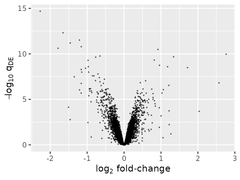
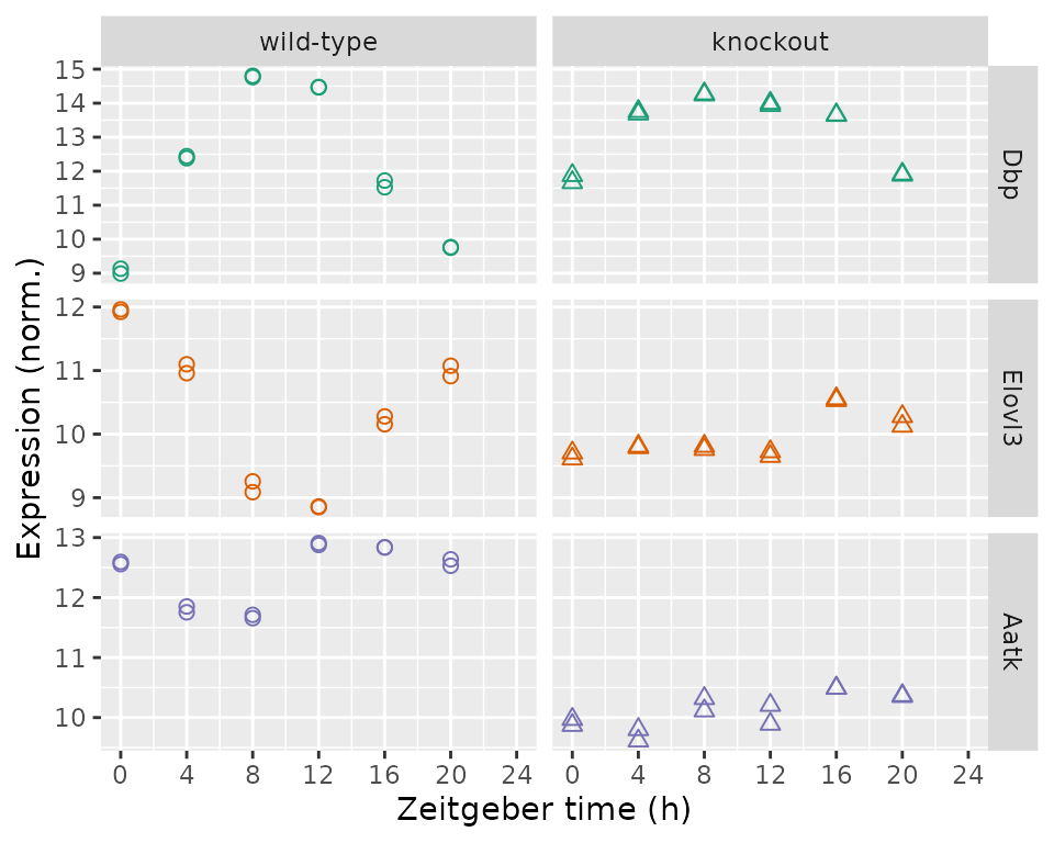
Another is a plot of expression as a function of time and genotype for individual genes. Here we show, from top to bottom, the top rhythmic gene, top differentially rhythmic gene, and top differentially expressed gene by q-value.
geneIdsNow = c(rhyLimmaSummary$gene_id[1L], drLimma$gene_id[1L], deLimma$gene_id[1L])
geneSymbolsNow = unname(getSYMBOL(geneIdsNow, 'org.Mm.eg.db'))

df = data.table(t(y[geneIdsNow, ]))
setnames(df, geneSymbolsNow)
df[, sample_id := colnames(y[geneIdsNow, ])]

df = merge(df, metadata[, .(sample_id, cond, time)], by = 'sample_id')
df = melt(df, measure.vars = geneSymbolsNow, variable.name = 'symbol',
          value.name = 'expr')
df[, symbol := factor(symbol, geneSymbolsNow)]

ggplot(df) +
  facet_grid(symbol ~ cond, scales = 'free_y') +
  geom_point(aes(x = time, y = expr, shape = cond, color = symbol), size = 2) +
  labs(x = 'Zeitgeber time (h)', y = 'Expression (norm.)') +
  scale_shape(solid = FALSE, guide = 'none') +
  scale_color_brewer(type = 'qual', palette = 'Dark2', guide = 'none') +
  scale_x_continuous(limits = c(0, 24), breaks = seq(0, 24, 4))